Recipes
Add Contextual Layers
ArcticDEM (NSIDC Sea Ice Polar Stereographic North, EPSG:3413)
Provided by Esri Polar/ArcticDEM ImageServer
m.add(IS2view.image_service_layer('ArcticDEM'))
Reference Elevation Model of Antarctica (Antarctic Polar Stereographic, EPSG:3031)
Provided by Esri Polar/AntarcticDEM ImageServer
m.add(IS2view.image_service_layer('REMA'))
Plot a Transect
Requires optional geopandas dependency.
import geopandas
# read shapefile of glacial flowlines
gdf = geopandas.read_file('/vsizip/shapefiles.zip/glacier0001.shp')
# add geodataframe
m.add_geodataframe(gdf)
# iterate over features
for feature in m.geometries['features']:
   ds.timeseries.plot(feature, cmap='rainbow', legend=True,
      variable=IS2widgets.variable.value,
   )
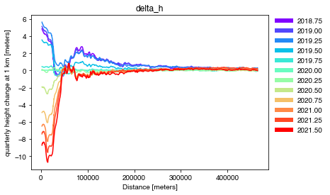
Fig. 2 Greenland glacier flowlines from Felikson et al. (2020)
Plot Multiple Time Series
Requires optional geopandas and fiona dependencies.
import fiona
fiona.drvsupport.supported_drivers['LIBKML'] = 'rw'
import geopandas
import numpy as np
import matplotlib.pyplot as plt
# read kml file with subglacial lake outlines
gdf = geopandas.read_file('lake_outlines.kml')
# add geodataframe of Whillians ice stream subglacial lakes
m.add_geodataframe(gdf[gdf['names'].str.startswith('Whillians')])
# create figure axis
fig, ax = plt.subplots()
fig.patch.set_facecolor('white')
# plot colors for each geometry
n_features = len(m.geometries['features'])
plot_colors = iter(plt.cm.rainbow_r(np.linspace(0,1,n_features)))
# iterate over features
for geo in m.geometries['features']:
   color = next(plot_colors)
   ds.timeseries.plot(geo, ax=ax,
      variable=IS2widgets.variable.value,
      color=color
   )
# show combined plot
plt.show()

Fig. 3 Antarctic subglacial lake delineations from Fricker et al. (2007)
Plot an Area Average
Requires optional geopandas dependency.
import geopandas
import matplotlib.pyplot as plt
# read Greenland basins
gdf = geopandas.read_file('Greenland_Basins_PS_v1.4.2.zip')
# reduce to NW region
subregion = 'NW'
region = gdf[gdf['SUBREGION1'] == subregion].dissolve(by='SUBREGION1')
region['NAME'] = f'{subregion} Greenland'
# add geodataframe
m.add_geodataframe(region)
# iterate over features
for feature in m.geometries['features']:
   ds.timeseries.plot(feature, legend=True,
      variable=IS2widgets.variable.value,
      color='mediumseagreen'
   )
# show average plot
plt.show()
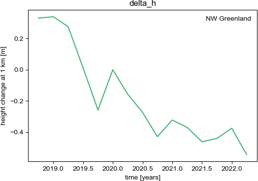
Fig. 4 Greenland drainage basins from Mouginot and Rignot (2019)
Calculate Area Averages
Requires optional geopandas dependency.
import geopandas
import numpy as np
import matplotlib.pyplot as plt
import matplotlib.colors as colors
# data release and variable
release = IS2widgets.release.value
variable = IS2widgets.variable.value
# read shapefile with drainage outlines
gdf = geopandas.read_file('IceBoundaries_Antarctica_v02.shp')
# get unique list of subregions
subregions = gdf[gdf['TYPE'] == 'GR']['Subregions'].unique()
# plot colors for each subregion
n_features = len(subregions)
plot_colors = iter(plt.cm.rainbow_r(np.linspace(0,1,n_features)))
# iterate over subregions
for subregion in sorted(subregions):
   # add geodataframe of drainages within subregion
   color = colors.to_hex(next(plot_colors))
   data = gdf[(gdf['TYPE'] == 'GR') & (gdf['Subregions'] == subregion)]
   m.add_geodataframe(data, style=dict(color=color))
   # allocate for combined area and volume
   area = np.zeros_like(ds.time, dtype=np.float64)
   volume = np.zeros_like(ds.time, dtype=np.float64)
   # iterate over features
   for geo in m.geometries['features']:
      ds.timeseries.extract(geo, variable=variable)
      # add to total area and volume
      area += ds.timeseries._area
      volume += ds.timeseries._area*ds.timeseries._data
   # create output figure
   fig, ax = plt.subplots()
   fig.patch.set_facecolor('white')
   ax.plot(ds.timeseries._time, volume/area)
   ax.set_xlabel('{0} [{1}]'.format('time', 'years'))
   ax.set_ylabel('{0} [{1}]'.format(ds.timeseries._longname, ds.timeseries._units))
   ax.set_title('{0} average {1}'.format(subregion,variable))
   # set axis ticks to not use constant offset
   ax.xaxis.get_major_formatter().set_useOffset(False)
   # save average plot
   plt.savefig(f'ATL15_{release}_{subregion}_{variable}.pdf')
   # drop features for subregion
   m.geometries['features'] = []
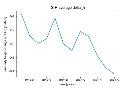
Fig. 5 MEaSUREs Antarctic Boundaries from Mouginot et al. (2017)
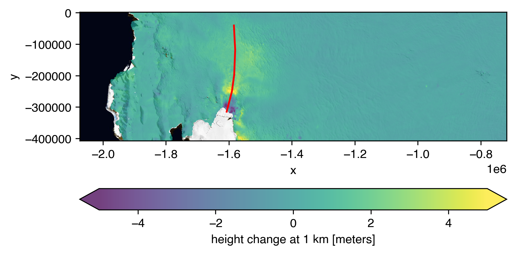
Save a Map to a File
Requires optional geopandas and owslib dependencies.
import matplotlib.pyplot as plt
# create a figure and axis
fig,ax = plt.subplots()
# create image of basemap
m.plot_basemap(ax=ax)
# create image of current map
ds.leaflet.imshow(ax=ax)
# add all geometries to the map
m.plot_geometries(ax=ax, color='red')
# save map plot
plt.savefig('map.png', bbox_inches='tight', dpi=300)
Remove Image Service Layer from Map
ds.leaflet.reset()